500 Mpc/h

Here we download and analyse the simulations produced in a simulation box of 500 Mpc/h in each direction.

import numpy as np
import matplotlib.pyplot as plt
import pickle, os
from glob import glob
from StoReS import *
import tools21cm as t2c
from tqdm import tqdm

N-body simulation with 500 Mpc/h in each direction

Cosmology of the simulation:

\(\Omega_\mathrm{m} = 0.27\), \(\Omega_\mathrm{b} = 0.044\), \(h_\mathrm{0} = 0.7\), \(\sigma_\mathrm{8} = 0.8\), \(n_\mathrm{s} = 0.96\)

We define the box length and the path to the folder for downloading the data.

box_len  = 500/0.7
save_dir = './work/'
eor_hist = {}

Density fields - 500 Mpc/h

N-Body (CUBEP3M) snapshots will be downloaded.

dn_url = 'https://ttt.astro.su.se/~gmell/500Mpc/densities/nc300/'
url_dict = {'dens': dn_url}
c2r = C2RAY(work_dir={'dens': save_dir+'density/'}, verbose=False)
c2r.set_links(url_dict)
zs = c2r.zs_dict['dens']
for i,z in tqdm(enumerate(zs)):
    dn, ff = c2r.get_density_data_z(z)
    # os.remove(ff)
print('Data saved in {}'.format(c2r.work_dir['dens']))

74it [00:05, 12.78it/s]

Data saved in ./work/density/

500Mpc/h Reionisation Simulation Suite

C2RMAX10

This simulation models the reionization process assuming spin saturation (\(T_{S}\gg T_{CMB}\)). is described in See Georgiev et al. (2022) the detailed description.

xf_url = 'https://ttt.astro.su.se/~gmell/500Mpc/500Mpc_z50_0_Rmax10_300/'
dn_url = 'https://ttt.astro.su.se/~gmell/500Mpc/densities/nc300/'
url_dict = {'xfrac': xf_url, 'dens': dn_url, }
c2r = C2RAY(work_dir={'dens': save_dir+'density/', 'xfrac': save_dir+'C2RMAX10/'}, verbose=False)
c2r.set_links(url_dict)
zs = np.intersect1d(c2r.zs_dict['xfrac'], c2r.zs_dict['dens'])
xs = []
for i,z in tqdm(enumerate(zs)):
    # print('{}/{}'.format(i+1,len(zs)))
    data = c2r.get_data_z(z)
    xf = data['xfrac']
    dn = data['dens']
    xs.append(xf.mean())
    # os.remove(data['xfrac_filename'])
    # os.remove(data['dens_filename'])
xs = np.array(xs)
eor_hist['C2RMAX10'] = {'z': zs, 'x': xs}
print('Data saved in {}'.format(c2r.work_dir['xfrac']))

70it [00:12,  5.59it/s]

Data saved in ./work/C2RMAX10/

C2LLS10

This simulation models the reionization process assuming spin saturation (\(T_{S}\gg T_{CMB}\)). is described in See Georgiev et al. (2022) the detailed description.

xf_url = 'https://ttt.astro.su.se/~gmell/500Mpc/500Mpc_z50_0_LLS10_300/'
dn_url = 'https://ttt.astro.su.se/~gmell/500Mpc/densities/nc300/'
url_dict = {'xfrac': xf_url, 'dens': dn_url, }
c2r = C2RAY(work_dir={'dens': save_dir+'density/', 'xfrac': save_dir+'C2LLS10/'}, verbose=False)
c2r.set_links(url_dict)
zs = np.intersect1d(c2r.zs_dict['xfrac'], c2r.zs_dict['dens'])
xs = []
for i,z in tqdm(enumerate(zs)):
    data = c2r.get_data_z(z)
    xf = data['xfrac']
    dn = data['dens']
    xs.append(xf.mean())
    # os.remove(data['xfrac_filename'])
    # os.remove(data['dens_filename'])
xs = np.array(xs)
eor_hist['C2LLS10'] = {'z': zs, 'x': xs}
print('Data saved in {}'.format(c2r.work_dir['xfrac']))

56it [00:10,  5.49it/s]

Data saved in ./work/C2LLS10/

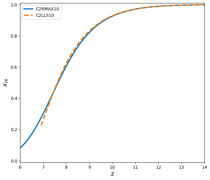
Reionization history of the above simulations

fig, ax = plt.subplots(1,1,figsize=(7,6))
# fig.suptitle('Georgiev et al. (2022)')
ax.plot(eor_hist['C2RMAX10']['z'], 1-eor_hist['C2RMAX10']['x'], lw=3, ls='-',  label='C2RMAX10')
ax.plot(eor_hist['C2LLS10']['z'], 1-eor_hist['C2LLS10']['x'], lw=3, ls='--', label='C2LLS10')
ax.set_xlabel('z', fontsize=14)
ax.set_ylabel('$x_\mathrm{HI}$', fontsize=14)
ax.legend()
ax.axis([6,14,-0.01,1.01])
plt.tight_layout()
plt.show()

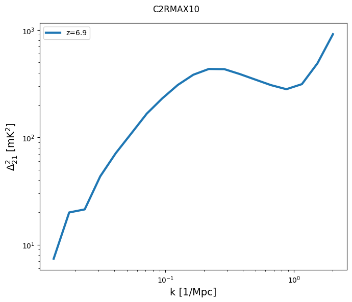
Power spectrum at z=6.9 from C2RMAX10

xf_url = 'https://ttt.astro.su.se/~gmell/500Mpc/500Mpc_z50_0_Rmax10_300/'
dn_url = 'https://ttt.astro.su.se/~gmell/500Mpc/densities/nc300/'
url_dict = {'dens': dn_url, 'xfrac': xf_url}

c2r = C2RAY(work_dir={'dens': save_dir+'density/', 'xfrac': save_dir+'C2RMAX10/'})
c2r.set_links(url_dict)
z = 6.905
data = c2r.get_data_z(z)
xf = data['xfrac']
dn = data['dens']

The file already exists.
The file already exists.

dt = t2c.calc_dt(xf, dn, z=z)
ps, ks = t2c.power_spectrum_1d(dt, kbins=20, box_dims=box_len)

fig, ax = plt.subplots(1,1,figsize=(7,6))
fig.suptitle('C2RMAX10')
ax.loglog(ks, ps*ks**3/2/np.pi**2, lw=3, ls='-',  label='z={:.1f}'.format(z))
ax.set_xlabel('k [1/Mpc]', fontsize=14)
ax.set_ylabel('$\Delta^2_\mathrm{21}$ [mK$^2$]', fontsize=14)
ax.legend()
# ax.axis([6,14,-0.01,1.01])
plt.tight_layout()
plt.show()